From profiling to production: How we reduced our log processing service's costs by 80%

A critical part of Merge’s infrastructure is its ability to persist API logs, which give customers visibility into their integrations. 

These logs (which are essentially payloads received from calls to 3rd party integrations) are sent to Elasticsearch for storage and querying. However, Elasticsearch has a hard limit on document size. To handle this, we have a service called the "Payload Trimmer."

The trimmer's job sounds simple: if a payload is too big, trim it down to size while preserving the most important data. But this service was a silent consumer of resources. It was running with a minimum of 125 Kubernetes pods, and with autoscaling, would often require even more during peak traffic. 

We knew there was an opportunity to optimize, but the first rule of optimization is: don't guess, measure.

This is the story of how we used a systematic, data-driven approach to performance tuning. It’s less about a single clever algorithm and more about a repeatable playbook that any engineer can use to hunt down and eliminate bottlenecks. The result? A 5x performance increase and an 80% reduction in our worker pod count.

{{this-blog-only-cta}}

The problem: how do you intelligently trim a JSON object?

Before diving into the code, let's define the problem more clearly. 

A JSON payload is essentially a tree structure of nested dictionaries (keys and values) and lists. Our goal is to reduce the total size of this tree by pruning its largest "leaf nodes"—the individual values (like long strings) at the end of each branch.

Our original PayloadTrimmer was designed to do this with a straightforward, four-step algorithm:

1. Traverse: Recursively walk the entire JSON tree.
2. Store: For every leaf node encountered, create a PayloadTrimmerNode object that stores the full path from the root of the tree to that leaf.
3. Sort: Collect all these node objects into a list and sort it by the size of the leaf value, from largest to smallest.
4. Pop & Replace: Iterate through the sorted list, and for each of the largest nodes, use its stored path to walk the tree again and replace the value with a placeholder string.

This initial approach intentionally prioritized clarity over performance. While this trade-off was acceptable early on, it became unsustainable as Merge's log volumes grew, prompting us to reevaluate our approach. Instead of rewriting it on a hunch, we followed a process to let the data guide us.

The investigator's toolkit: an intro to Python profilers

To find our bottleneck, we used two standard Python profiling tools. Understanding what they do is key to following the investigation.

• cProfile: This is Python's built-in statistical profiler. It gives you a high-level, function-by-function breakdown of where your program is spending its time. It tells you how many times each function was called and the total time spent within it. It's the perfect tool for getting a 10,000-foot view to identify which general areas of your code are slow.
• line_profiler: This is a third-party library that provides line-by-line profiling. After cProfile points you to a slow function, line_profiler is the magnifying glass you use to examine every single line within that function to see exactly which one is the culprit. You typically use it by adding a @profile decorator to the function you want to inspect.

The Playbook in action: from smoke to smoking gun

Armed with our tools, we began the hunt.

Step 1: The 10,000-Foot View with cProfile

We started with cProfile to get a high-level map of where our code was spending its time. The results immediately told a compelling story. We could see a clear chain of command where the cost flowed from our main entrypoint function into a recursive traversal function, which in turn spent most of its time in a helper function responsible for creating new nodes. This gave us our primary suspect and a clear direction: the bottleneck was related to how we were creating state during our recursive traversal.

Step 2: following the Smoke with line_profiler

 With cProfile having pointed to the smoke, we grabbed our "magnifying glass," line_profiler, to find the fire. We profiled the same code again, but this time with line_profiler, which gave us a detailed, line-by-line report for the functions we were interested in.

First, we aimed it at our main entrypoint function. The profiler showed that nearly all of the execution time—a staggering 94.5%—was spent inside the call to our recursive helper function. This confirmed that the logic within the main function was not the problem.

This is a critical first step in any investigation: ignore the noise and find the real hotspot. We now knew we didn't have to analyze the entire class, just that one recursive function.

Step 3: pinpointing the smoking gun

The profiler output for the recursive function narrowed the search even further. It revealed that the most time-consuming lines were not the recursion itself, but the calls to a helper function that created a new node for each step of the traversal. So, we ran line_profiler one more time, aimed squarely at spawn_new_node. The result was the smoking gun.

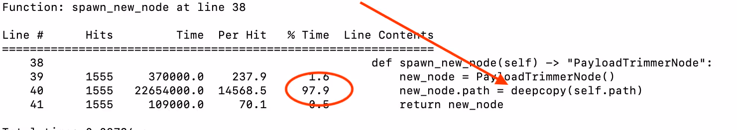
It was clear as day. A single line of code was responsible for 97.9% of the function's execution time: new_node.path = deepcopy(self.path)

We had found our bottleneck. The investigation was over, and the real work could begin.

From diagnosis to cure: attacking the root cause

This deep dive revealed two common Python performance anti-patterns that are great lessons for any engineer.

1. The deepcopy trap

deepcopy is a powerful tool, but it's incredibly expensive. To create a "deep" copy, it has to recursively traverse every level of an object and create a brand-new, independent copy of every element. On a hot path—a piece of code that is executed thousands or millions of times—this cost adds up exponentially. Our code was calling it for every single leaf in the payload, which was the source of our performance woes.

Lesson: Be extremely wary of deepcopy in loops or recursive functions. Ask yourself if there’s a way to achieve your goal without creating full copies of your data.

2. Mutable objects vs. immutable tuples

The root cause of our deepcopy usage was our choice of data structure: a mutable list (self.path) inside a mutable custom object (PayloadTrimmerNode). To prevent different nodes from accidentally modifying the same path list as it was passed down through the recursion, we were forced to make expensive copies.

The solution was to switch to a simple, immutable data structure: a tuple. The new implementation traverses the payload and generates a simple list of tuples, where each tuple contains (size, parent_reference, key_or_index).

This change had profound performance implications:

• Eliminated copying: Because tuples are immutable, they can be passed around freely without fear of accidental modification. This completely removed the need for deepcopy
• Memory efficiency: Immutable objects like tuples have a fixed structure. This allows Python to store them more compactly in memory compared to mutable objects, which need to reserve extra space for potential additions. This compact layout means better cache utilization and faster retrieval
• Direct access: Instead of storing a "path" and re-walking the tree, we now had a direct reference to the parent object. The replacement became a single, blazing-fast operation: parent_reference[key_or_index] = "[TRUNCATED]"

Lesson: Favor immutable data structures like tuples on performance-critical paths. Their memory layout is more efficient, and they can help you avoid complex state management and the need for expensive defensive copies.

The system-wide payoff: thinking in terms of Amdahl's Law

After achieving a 5x speedup in our trimming function, I was excited to see the impact on our production system. I deployed the change and watched the dashboards. 

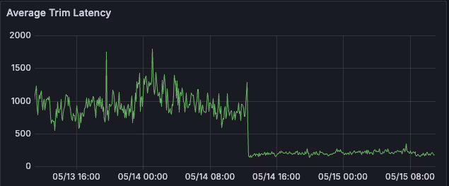
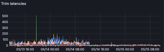
Just as expected, our "Trim Latency" metric plummeted. A huge success! But then I looked at the most important metric: the length of our processing queue. It hadn't budged.

Despite the massive local win, the system as a whole wasn't processing logs any faster. This is where a key concept in systems performance comes into play: Amdahl's Law.

Amdahl's Law states that the overall performance improvement gained by optimizing a single part of a system is limited by the fraction of time that the improved part is actually used. 

In our case, the time to process a batch of logs can be modeled as:

t_total = t_trim + t_overhead

Here's the breakdown:

• t_trim is the "fraction of time the improved part is used"—the time spent running our Python trim function.
• t_overhead is the separately optimizable part. For us, this included fetching from the queue, network I/O, and most importantly, a fixed batch size and a hardcoded sleep(2) interval.

These weren't arbitrary numbers; they were critical safety measures. The batch size and sleep interval worked together to prevent our old, resource-intensive code from overwhelming the CPU and memory on the worker pods, and to pace the requests to our Elasticsearch cluster so it wouldn't get flooded.

My initial optimization had slashed t_trim so effectively that it was no longer a significant part of the equation:

t_new_total = (t_trim/5) + t_overhead ≈ t_overhead

The initial puzzle was solved. Our t_overhead was completely overshadowing the gains from the code optimization. The system was now spending almost all its time waiting on the sleep(2) interval and network I/O, which both had become the new bottlenecks. The key insight, however, was that our new code was so efficient that these strict safety limits were no longer necessary. A worker could now process a much larger batch in far less time without straining its resources.

With this understanding, the path forward was clear. We had to attack the overhead. We carefully experimented with tuning the system's configuration, ultimately reducing the sleep time and increasing our batch size.

This was the change that finally bent the curve. With the overhead reduced, the speed of the now-optimized trim function could finally shine through, and our overall system throughput skyrocketed.

Now we had a different, much better problem: the system was too fast. To bring our processing speed back to the desired level that our downstream services were comfortable with, we could finally reduce the number of workers. 

We tested this hypothesis carefully, monitoring queue depth and Elasticsearch load, and gradually scaled down our deployment. The result? A new minimum pod count of 25—an 80% reduction in compute cost, achieved not just by optimizing code, but by understanding and tuning the entire system around it.

Key takeaways

This project was a powerful reminder of several key engineering principles:

1. Profile, don't guess: Standard tools like cProfile and line_profiler are invaluable for turning hunches into data-driven action.
2. Mind your data structures: The shift from mutable objects to immutable tuples was the core of the performance gain. Often, the biggest wins come from rethinking data representation
3. Connect local wins to system-wide impact: Understanding how your code fits into the larger system (using frameworks like Amdahl's Law) is crucial for turning a local optimization into a global one.
4. Optimization is an iterative process: Profile, optimize, measure, repeat. This cycle ensures you're always working on the most impactful parts of the code.

By following this process, we were able to deliver a huge win for our platform's efficiency and cost, all starting from a single, targeted code optimization.

{{this-blog-only-cta}}